Sky model tutorial¶

Accessing the Cosmoglobe sky model¶

To access the Cosmoglobe sky model, we will use the cosmoglobe.sky_model function. This function initializes the Cosmoglobe sky model at a requested nside. The first time this function is called a 800MB minimal Commander chain file containing the model data is downloaded and cached.

[26]:

import cosmoglobe
model = cosmoglobe.sky_model(nside=256)

Initializing model from cached chainfile

synch: 100%|█████████████████████████████████| 6/6 [00:04<00:00,  1.32it/s]

For people working with Commander3, a custom sky model can be initialized given an arbitrary Commander3 chain file using the cosmoglobe.sky_model_from_chain function.

[28]:

import cosmoglobe

chain = "path/to/commander3_chain.h5"
model = cosmoglobe.sky_model_from_chain(chain, nside=256)

Initializing model from chain_test.h5

synch: 100%|█████████████████████████████████| 6/6 [00:04<00:00,  1.33it/s]

Inspecting the model¶

To get an overview of the model and the sky components in it, we can print the model object:

[29]:

model

[29]:

SkyModel(
  version: BeyondPlanck
  nside: 256
  components(
    (ame): SpinningDust(freq_peak)
    (cmb): CMB()
    (dust): ModifiedBlackbody(beta, T)
    (ff): LinearOpticallyThin(T_e)
    (radio): AGNPowerLaw(alpha)
    (synch): PowerLaw(beta)
  )
)

Model components¶

Let us explore the sky components in further detail. Each component can be individually accessed through the attribute names seen in the parentheses of the print(model) output.

[30]:

print(model.components["dust"])
print(model.components["synch"])

ModifiedBlackbody(beta, T)
PowerLaw(beta)

Component attributes¶

The model data is stored in the following component attributes:

amp: Amplitude map at the reference frequency (Commander average posterior map)
freq_ref: Reference frequency of amp
spectral_parameters: A dictionary containing the spectral parameters

We can print these attributes:

[31]:

print(model.components["dust"].amp)
print(model.components["dust"].freq_ref)
print(model.components["dust"].spectral_parameters)

[[30.30987493 -0.43109241  8.45230192 ...  6.66705892  9.97193761
  11.8158503 ]
 [-4.01957718 -1.29835574  1.69922271 ...  4.33198759 -5.62753956
   0.72578835]
 [ 2.61048442  2.11811903 -0.90430579 ... -6.73241148  0.47604929
   0.76062461]] uK_RJ
[[545.]
 [353.]
 [353.]] GHz
{'beta': <Quantity [[1.54764616],
           [1.57661884],
           [1.57661884]]>, 'T': <Quantity [[17.33100722],
           [17.33100722],
           [17.33100722]] K>}

Visualizing components¶

The maps of a component (amp or a spectral parameter map) can be visualized like normal using healpy.mollview.

Alternatively, we can use cosmoglobe.plot, which is a wrapper on healpy’s mollview function that features built-in esthetique choices.

In this tutorial we will use cosmoglobe.plot. For a more in in-depth overview of the built-in plot function, please see the plotting tutorial (coming soon).

[32]:

from cosmoglobe import plot
from healpy import mollview
%matplotlib inline
path = "/Users/metinsan/Documents/doktor/Cosmoglobe_test_data/" # datapath

Let us plot some of the reference amplitude maps used in the current model:

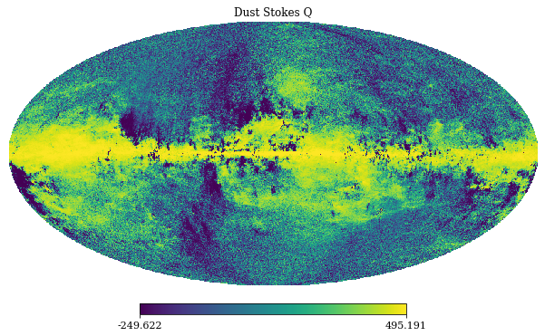
[33]:

# Stokes Q map of dust
dust_amp_Q = model.components["dust"].amp[1]
mollview(
    dust_amp_Q,
    title='Dust Stokes Q',
    norm="hist",
)

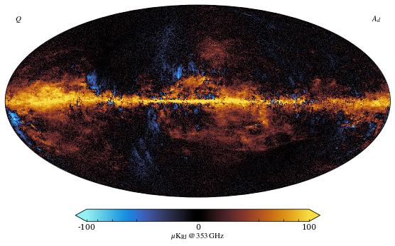
Or use the cosmoglobe “plot” function for direct plotting and formatting of a model. This function can be used in the same way as mollview, and is a wrapper on the healpy projview function with some extra features.

[34]:

# Pass in the model and specify which component to plot.
plot(model, comp="dust", sig="Q",)

[34]:

(<matplotlib.collections.QuadMesh at 0x7f804a7b1070>,
 {'data': array([-4.01957718, -1.29835574,  1.69922271, ...,  4.33198759,
         -5.62753956,  0.72578835]),
  'comp': 'dust',
  'sig': 1,
  'rlabel': '$A_d$',
  'llabel': '$Q$',
  'unit': '$\\mu\\mathrm{K}_{\\mathrm{RJ}}\\,@\\,353\\,\\mathrm{GHz}$',
  'ticks': [-100, 0, 100],
  'min': None,
  'max': None,
  'rng': None,
  'norm': 'symlog2',
  'norm_dict': {'linthresh': 5},
  'cmap': 'iceburn',
  'freq_ref': <Quantity 353. GHz>,
  'width': 8.302200083022,
  'nside': 256,
  'ticklabels': ['$-100$', '$0$', '$100$']})

Simulations¶

The primary use case of the cosmoglobe software is to provide the community with astrophysical maps generated with the Cosmoglobe Sky Model. The mean posterior maps used in the sky model (given at some reference frequency) are directly accessible through model attributes as demonstrated in the above section.

These maps can additionally be extrapolated to arbitrary frequencies to produce simulations of the sky. In the following we look at how we can use cosmoglobe to generate full sky simulations:

Simulating component emission¶

We can simulate the emission from a component at an arbitrary frequency freq by calling the component’s __call__ method, e.g, model.dust(freq).

This function takes in the following key word arguments:

freqs : A frequency, or a list of frequencies for which to evaluate the sky emission
bandpass : Bandpass profile corresponding to the frequencies (optional)
fwhm : The full width half max parameter of the Gaussian used to smooth the output (optional)
output_unit : The output units of the emission (By default the output unit of the model is always in uK_RJ

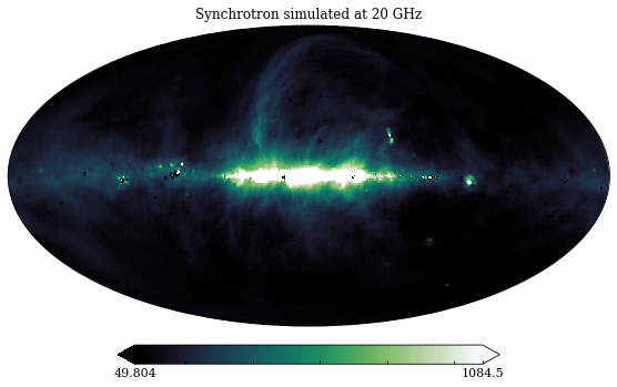
Below, is a simulation of synchrotron emission at \(20\;\mathrm{GHz}\):

[35]:

import astropy.units as u  # astropy.units is a package for unit handling

# Simulated synchrotron emission at 20GHz
simulated_emission = model(20*u.GHz, components=["synch"])

plot(
    simulated_emission[0],
    title='Synchrotron simulated at 20 GHz',
    cmap='swamp',
)

[35]:

(<matplotlib.collections.QuadMesh at 0x7f8020251670>,
 {'data': array([93.58164725, 90.38146853, 85.50231773, ..., 76.24776625,
         78.24186881, 79.20658964]),
  'comp': None,
  'sig': 0,
  'rlabel': None,
  'llabel': None,
  'unit': None,
  'ticks': [49.80404939854137, 1084.5020392865435],
  'min': None,
  'max': None,
  'rng': None,
  'norm': None,
  'norm_dict': None,
  'cmap': 'swamp',
  'freq_ref': None,
  'width': 8.302200083022,
  'nside': 256,
  'ticklabels': ['$49$', '$1084$']})

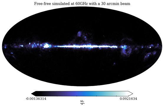
And a simulation of free-free emission at \(20\;\mathrm{GHz}\) with a FWHM of \(30\;'\) and output units set to \(\mathrm{MJy/sr}\):

[36]:

# Simulated free-free emission at 60GHz seen by a 30 arcmin
# beam in units of MJy/sr
simulated_emission = model(
    60*u.GHz,
    fwhm=30*u.arcmin,
    output_unit='MJy/sr',
    components=["ff"]
)

plot(
    simulated_emission[0],
    title='Free-free simulated at 60GHz with a 30 arcmin beam',
    unit=simulated_emission.unit,
    cmap='freeze',
)

[36]:

(<matplotlib.collections.QuadMesh at 0x7f802016db80>,
 {'data': array([ 1.05682988e-04, -5.59499953e-05, -1.05648426e-04, ...,
         -1.31944092e-03, -1.22261591e-03, -1.15828253e-03]),
  'comp': None,
  'sig': 0,
  'rlabel': None,
  'llabel': None,
  'unit': '$\\mathrm{\\frac{MJy}{sr}}$',
  'ticks': [-0.0013631425254432069, 0.0921634371558297],
  'min': None,
  'max': None,
  'rng': None,
  'norm': None,
  'norm_dict': None,
  'cmap': 'freeze',
  'freq_ref': None,
  'width': 8.302200083022,
  'nside': 256,
  'ticklabels': ['$-0.0$', '$0.09$']})

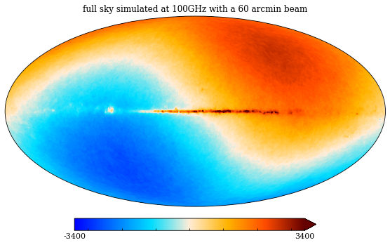
Simulating model emission¶

Similarly, by calling the model’s __call__ function (which takes in the same keyword arguments), we can simulate the sky emission over the full model at a given frequency:

[37]:

# Simulated full sky emission at 100GHz seen by a 60 arcmin
# beam in units of uK_RJ
simulated_emission = model(100*u.GHz, fwhm=60*u.arcmin)

plot(
    simulated_emission[0],
    title='full sky simulated at 100GHz with a 60 arcmin beam',
    min=-3400,
    max=3400,
)

[37]:

(<matplotlib.collections.QuadMesh at 0x7f7fc856b4f0>,
 {'data': array([ 1857.06100303,  1854.47363061,  1871.76044276, ...,
         -1952.45172834, -1940.09037429, -1936.28452927]),
  'comp': None,
  'sig': 0,
  'rlabel': None,
  'llabel': None,
  'unit': None,
  'ticks': [-3400, 3400],
  'min': -3400,
  'max': 3400,
  'rng': None,
  'norm': None,
  'norm_dict': None,
  'cmap': 'planck',
  'freq_ref': None,
  'width': 8.302200083022,
  'nside': 256,
  'ticklabels': ['$-3400$', '$3400$']})

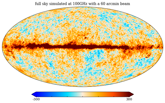
It is possible to remove the solar dipole from the model, by calling model.cmb.remove_dipole():

[38]:

# Remove the solar dipole
model.remove_dipole()

# Simulated full sky emission at 100GHz seen by a 60 arcmin
# beam in units of uK_RJ
simulated_emission = model(100*u.GHz, fwhm=60*u.arcmin)

plot(
    simulated_emission[0],
    title='full sky simulated at 100GHz with a 60 arcmin beam',
    min=-300,
    max=300,
)

[38]:

(<matplotlib.collections.QuadMesh at 0x7f8056c5cbe0>,
 {'data': array([-76.37011282, -79.74717809, -70.26625067, ...,  11.3845686 ,
          15.94003791,  20.53557578]),
  'comp': None,
  'sig': 0,
  'rlabel': None,
  'llabel': None,
  'unit': None,
  'ticks': [-300, 300],
  'min': -300,
  'max': 300,
  'rng': None,
  'norm': None,
  'norm_dict': None,
  'cmap': 'planck',
  'freq_ref': None,
  'width': 8.302200083022,
  'nside': 256,
  'ticklabels': ['$-300$', '$300$']})

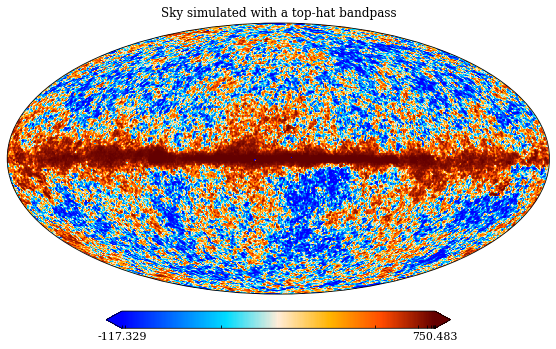
Bandpass integration¶

We can also make simulations that have integrated the sky emission over a given bandpass. By default if only a list of frequencies are supplied without an explicit bandpass input, a top-hat bandpass will be used during the integration.

[39]:

import numpy as np

frequencies = np.arange(100, 110, 50)*u.GHz

simulated_emission = model(frequencies, fwhm=40*u.arcmin)

plot(
    simulated_emission[0],
    title='Sky simulated with a top-hat bandpass',
    norm='hist',
)

[39]:

(<matplotlib.collections.QuadMesh at 0x7f804ff81040>,
 {'data': array([-69.07164031, -80.50819514, -74.77978502, ...,  21.37857762,
          35.67817327,  39.27271206]),
  'comp': None,
  'sig': 0,
  'rlabel': None,
  'llabel': None,
  'unit': None,
  'ticks': [-117.32857341383954, 750.4833935506042],
  'min': None,
  'max': None,
  'rng': None,
  'norm': 'hist',
  'norm_dict': None,
  'cmap': 'planck',
  'freq_ref': None,
  'width': 8.302200083022,
  'nside': 256,
  'ticklabels': ['$-117$', '$750$']})

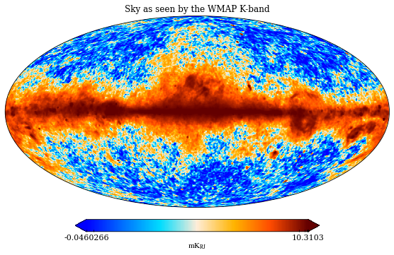
In the following we use the WMAP K-band bandpass profile:

[46]:

bandpass = path+"wmap_bandpass.txt"
frequencies, bandpass, _ = np.loadtxt(bandpass, unpack=True)

#add astropy units to the bandpass
frequencies*= u.GHz
bandpass *= u.Unit("K_RJ")

Note that when we are working with bandpasses, we give the bandpass unit (even if it is normalized) to differentiate bandpasses measured in K_CMB and K_RJ units. Importing the cosmoglobe model allow us to use u.Unit("K_RJ") and u.Unit("K_CMB") to explicitly state which unit we need.

[47]:

# Note: Solar dipole is removed from the model
wmap_kband_emission = model(
    frequencies,
    bandpass,
    fwhm=0.88*u.deg,
    output_unit='mK_RJ'
)

plot(
    wmap_kband_emission[0],
    title='Sky as seen by the WMAP K-band',
    unit=wmap_kband_emission.unit,
    norm='hist',
)

[47]:

(<matplotlib.collections.QuadMesh at 0x7f8052702cd0>,
 {'data': array([-0.0069367 , -0.02060602, -0.01526639, ...,  0.02398448,
          0.03608212,  0.04311066]),
  'comp': None,
  'sig': 0,
  'rlabel': None,
  'llabel': None,
  'unit': '$\\mathrm{mK_{{RJ}}}$',
  'ticks': [-0.04602656430781337, 10.310317464575249],
  'min': None,
  'max': None,
  'rng': None,
  'norm': 'hist',
  'norm_dict': None,
  'cmap': 'planck',
  'freq_ref': None,
  'width': 8.302200083022,
  'nside': 256,
  'ticklabels': ['$-0.05$', '$10$']})

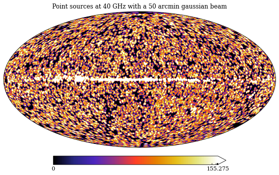
Point sources¶

The radio component does not store HEALPIX amplitude maps internally. Instead, the amp quantity contains a list of amplitude values, one per point source. Each source is then mapped to a HEALPIX map with a truncated gaussian beam whenever the model (or radio component) is called.

[42]:

# Point sources seen at 40GHz over a 50 arcmin gaussian beam
simulated_emission = model(30*u.GHz, fwhm=50*u.arcmin, components=["radio"])

plot(
    simulated_emission[0],
    title='Point sources at 40 GHz with a 50 arcmin gaussian beam',
    norm='hist',
    cmap='CMRmap'
)

[42]:

(<matplotlib.collections.QuadMesh at 0x7f80548037c0>,
 {'data': array([0.03262944, 0.06934092, 0.06042835, ..., 0.11145901, 0.025511  ,
         0.06111052]),
  'comp': None,
  'sig': 0,
  'rlabel': None,
  'llabel': None,
  'unit': None,
  'ticks': [0.0, 155.27530458805415],
  'min': None,
  'max': None,
  'rng': None,
  'norm': 'hist',
  'norm_dict': None,
  'cmap': 'CMRmap',
  'freq_ref': None,
  'width': 8.302200083022,
  'nside': 256,
  'ticklabels': ['$0$', '$155$']})

Plotting¶

In addition to the features already displayed previously in this tutorial, the plot function has a lot more new functionality.

Similar to available plotting scripts such as healpy’s mollview, plot allows for direct plotting of map-arrays. However, it also supports direct plotting of cosmoglobe model objects and direct reading of fits files.

Another defining feature of the code is the automatic parameter setting defined specifically for each sky component for the ultimate viewing pleasure, set by specifying the comp input.

Other useful features include direct smoothing, ud_grading and mono-dipole removal of the passed maps.

Here are some examples:

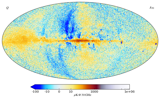
[43]:

plot(model, freq=30*u.GHz, sig="Q")

[43]:

(<matplotlib.collections.QuadMesh at 0x7f804e9cc9a0>,
 {'data': array([ -5.10686449,  12.55576019,  -3.41984734, ..., -17.241101  ,
          20.72343412,  -2.33641607]),
  'comp': 'freqmap',
  'sig': 1,
  'rlabel': '$A_{30}$',
  'llabel': '$Q$',
  'unit': '$\\mu\\mathrm{K}\\,@\\,30\\,\\mathrm{GHz}$',
  'ticks': [-100.0, -10, 0, 10, 1000.0, 1000000.0],
  'min': None,
  'max': None,
  'rng': None,
  'norm': 'symlog2',
  'norm_dict': None,
  'cmap': 'planck_log',
  'freq_ref': <Quantity 30. GHz>,
  'width': 8.302200083022,
  'nside': 256,
  'ticklabels': ['$-100$', '$-10$', '$0$', '$10$', '$1000$', '$10^{6}$']})

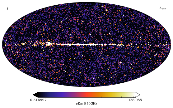
[44]:

plot(model, comp="radio", fwhm=30*u.arcmin)

[44]:

(<matplotlib.collections.QuadMesh at 0x7f805280e970>,
 {'data': array([-0.31644916, -0.11476952, -0.3912375 , ...,  0.01459645,
          0.10885113, -0.0720675 ]),
  'comp': 'radio',
  'sig': 0,
  'rlabel': '$A_{\\mathrm{ptsrc}}$',
  'llabel': '$I$',
  'unit': '$\\mu\\mathrm{K}_{\\mathrm{RJ}}\\,@\\,30\\,\\mathrm{GHz}$',
  'ticks': [-0.31699661232736154, 128.0551097852748],
  'min': None,
  'max': None,
  'rng': None,
  'norm': 'symlog2',
  'norm_dict': {'linthresh': 5},
  'cmap': 'CMRmap',
  'freq_ref': <Quantity 30. GHz>,
  'width': 8.302200083022,
  'nside': 256,
  'ticklabels': ['$-0.32$', '$128$']})

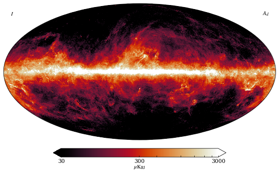
[45]:

fits_filename = path+"dust_c0001_k000200.fits"
plot(fits_filename, comp="dust")

[45]:

(<matplotlib.collections.QuadMesh at 0x7f8056cf99a0>,
 {'data': array([20.05815479,  7.049298  ,  3.61007396, ..., 22.9471769 ,
         17.30836798, 21.17100985]),
  'comp': 'dust',
  'sig': 0,
  'rlabel': '$A_d$',
  'llabel': '$I$',
  'unit': '$\\mu\\mathrm{K}_{\\mathrm{RJ}}$',
  'ticks': [30, 300, 3000],
  'min': None,
  'max': None,
  'rng': None,
  'norm': 'symlog2',
  'norm_dict': {'linthresh': 5},
  'cmap': 'sunburst',
  'freq_ref': 545.0,
  'width': 8.302200083022,
  'nside': 1024,
  'ticklabels': ['$30$', '$300$', '$3000$']})

Tutorials

Plotting tutorial